[컴선설] Lec 01 Linear Algebra

1. Linear Transformation

• Linear Transformation : $A{\mathbf x}={\mathbf b}$ form.
• Three cases : No solution / One solution / Infinite numbers of solution

Case A : No solution

• Given point ${\mathbf b}$ is not included in set of points spanned by $\mathbf {c_1, c_2, c_3}$
• Column vectors are not independent of each other
• $C(A)=\text{span}(A), {\mathbf b} \notin C(A)$

Case B : One solution

• ${\mathbf b} \in C(A), N(A)={\mathbf 0}$
• Column vectors are independent of each other.

Case C : Infinite solutions

• ${\mathbf b} \in C(A), N(A)\neq{\mathbf 0}$
• Column vectors are not independent of each other

2. Least Squares Method

• If the vector ${\mathbf b}$ not included in area spanned by column vectors, there’s no exact solution.
• Can find orthogonal projection $\hat {\mathbf b}$ to solve $A\hat {\mathbf x} = \hat {\mathbf b}$
• $\hat {\mathbf x}$ is least square solution of the $A{\mathbf x}={\mathbf b}$

2.1 Vector space

• = set of vectors
• 연산에 대해 닫혀있다 개념
• $\alpha {\mathbf a} + \beta {\mathbf b} = {\mathbf c}$ : for $\forall \alpha, \beta \in \R$
• Must include origin ($\mathbf 0$) to be a vector space

Span (or spanning set)

• ${\mathbf a}, {\mathbf b}$ 에 대해 $\alpha \mathbf a + \beta \mathbf b$ : Spanning set

3. Basis vector

• basis : vectors of the ‘minimum number’ that spans all points in original space

How to check linear independence

• given vector $\bf e_1, \bf e_2$, if there only exists trivial solution to $\alpha \bf e_1 + \beta \bf e_2 = 0$ ($\alpha = \beta = 0)$, $\bf e_1, \bf e_2$ are linearly independent

4. Find all solutions to linear system

Find Nullspace solution of Ax=b

• Find nullspace of matrix $A$
• $A \bf x =b$, $A\bf x = b+0=b$
• $\bf x_{complete} = x_{particular} + x_{null}$
• Using Gauss-Jordan Elimination → Pivot column을 non-pivot column으로 나타내기
• Number of pivot → rank / number of columns - rank = nullity (dimension of nullspace)

Find Complete solution of Ax=b

• solve with $\bf b$
• substitute 0 to null-space solution

5. Sub-space

• subset of original space. must include the origin

6. Elementary Matrix

• Matrix that expreses one elementary row operation
  1. 두 행 swap : Inverse는 자기자신 (Permutation matrix)
  2. 한 행에 다른 행의 scalar 배를 더하기 : Inverse는 다시 -scalar배 더한 elementary matrix
  3. 각 행을 scalar배 하기 : Inverse는 1/scalar배 하기
• determinent=1. swap한 경우만 -1

7. Gauss-Jordan Elimination

• RREF (Reduced Row Echelon Form) - Every pivot must be 1, pivot row must be zero except for the pivot

Gauss Jordan :
1. Make RREF
for column c:
  swap nonzero pivot row to c
  Multiply elementary matrix to remove value below pivot
  make pivot value 1
  make non-pivot value of the column zero
2. Solve nullspace solution
Solve RREF with Ax=0
remove pivot column value by substitution
3. Solve particular solution
solve for Ax=0
set non-pivot value 0

8. LU Decompositon

• Multiplying Elementry matrix on the left side of A makes it Upper triangular matrix
• $E_3E_2E_1Ax = UAx= E_3E_2E_1b$
• Let $L_{-1}=E_3E_2E_1$, $A=LU$
• $A=LU, LUx= b$
• $L{\bf y} = \bf b$ → Forward substitution
• $U{\bf x} = {\bf y}$ → Backward substitution

<LUdecomposition>
Procedure : 
set pivot[i] = i
for column k :
  find value in column k
  swap
  factor <- Aik / Akk
  Aik <- factor
  for row j=k+1 :
    Aij -= factor * Akj
 <LUsolve>
 for row i:
   sum = b[i]
   for column j=i+1 :
     sum -= Aij * x[j]
   x[i] = sum
 for row i=n-1 decreasing :
   sum = x[i]
   for column j=i+1 :
     sum-=Aij * x[j]
   x[i]=sum/Aii
 return x[i]

9. Four fundamental Subspace

• $C(A)$ : Column space, spanned by linearly independent column vectors
• $N(A)$ : Nullspace, spanning set that satisfies $A{\bf x} = {\bf 0}$
• $R(A) = C(A^T)$ : Row space, spanned by linearly indepenedent row vectors (or Column space of $A^T$
• $\text{dim}C(A) = \text{dim}C(A) = \text{dim}R(A^T)=r$ (Rank of A)
• $\text{dim}N(A) = \text{nullity}(A) = n-r$ ( # of column - rank)
• $\text{dim}N(A^T) = \text{nullity}(A^T) = m-r$ (# of row - rank)
• Rank-nullity theorem : $\dim C(A) + \dim N(A) = \dim V$ : dimension of domain
• Also $\dim C(A^T) + \dim N(A^T) = \dim W$ : dimension of codomain
• $C(A) \perp N(A^T)$
• $C(A^T) \perp N(A)$

10. Rank 1 matrix

• All column (or row) lies along the same line : $\text{rank}(A) = 1$

11. Trace

• summation of diagonal terms = sum of eigenvalues
• $\text{tr}(A) = \sum \lambda_i$

12. Symmetric matrix

Properties

• Eigenvalues of symmetric matrix are real.
• Every real matrix $A$ can be diagonalized by an orthogonal matrix $Q$
• $A=QDQ^T$, ($Q^TQ=I$)
• Symmetry of quadratic form : ${\bf x^T}A {\bf x}$ is real scalar for real vector $\bf x$
• Positive-definiteness : if eigenvalues of $A $ are strictly positive, → positive definite, ${\bf x^T}A{\bf x}>0$ for all nonzero $\bf x$

13. QR Factorization (decompositon)

• $A = QR$
• $Q$ : orthogonal (or unitary) matrix where $Q^T Q = I$ or $Q^*Q=I$
• $R$ : upper triangular matrix

Application

• Find least squares problem $\min_x \vert\vert A{\bf x} - {\bf b} \vert\vert $ can be solved using QR factorization
• $QRx \approx b$, $Q^TQRx = Rx=Q^Tb$
• Numerical stability : preserves length and angles
• Easy to apply on Iterative Methods

Classical Gram-schmidt

1. Takes columns of $A$, say $\bf a_1,a_2, \cdots, a_n$
2. Orthogonalize them step by step

\[{\bf q_1} = {\bf a_1 \over ||{\bf a_1}||}, {\bf q_2} = {\bf a_2 - \text{proj}_{\bf q_1}({\bf a_2}) \over ||{\bf a_1}||}\]

1. Collect the normalized orthogonal vectors as columns of $Q$.
2. Figure $R$ by computing $R= Q^TA$
   • To handle numerical stability and to solve ill-conditioned matrix, use Householder matrix
   • Provides stable way to work with systems without forming normal equations $A^TA$

Gram schmidt (Or QR Factorization)
1. Take columns of A, say a1, a2, ..., an
2. let q1 = a1 / |a1|, r11 = |a1|
3. let q2 = a2-(q1*a2)q1 / | a2-(q1*a2)q1 |, 
   r12 = q1*a2, r22 = | a2-(q1*a2)q1 |
4. let q3 = a3-(q1*a3)q1-(q2*a3)q2 / | a3-(q1*a3)q1-(q2*a3)q2 |
   r13 = q1*a3, r23 = q2*a3, r33 = | a3-(q1*a3)q1-(q2*a3)q2 |

Shapes and Dimensions of QR

• $A (m\times n) = Q(m \times m)R(m\times n)$ : Full decomposition
• $A(m\times n) = Q_{reduced}(m\times n) R_{top}(n\times n)$ : economy-sized decomposition
• Example!

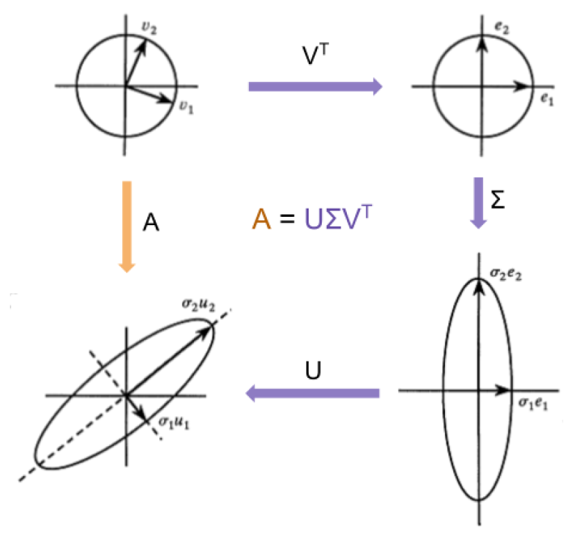
14. Singular Value Decomposition (SVD)

• For any real valued matrix $A (m \times n)$

\[A = U\Sigma V^T\]

where

1. $U (m\times m)$ orthogonal (or unitary) matrix, $U^TU=I_{m\times m}$ (Left singular vectors of $A$)
2. $\Sigma(m\times n)$ diagonal-like matrix (rectengular, only the diagonal terms are nonzero, singular values with descending order) $\sigma_1 \geq \sigma_2 \geq \cdots \geq 0$
3. $V(n\times n)$ orthogonal (or unitary) matrix, $V^TV = I_{n\times n}$. Columns of $V$ are right singular vectors of $A$

Properties of SVD

• Singular values
  • The numbers $\sigma_1, \sigma_2, \cdots$ on the diagonal of $\Sigma$
  • Nonnegative and arranged in descending order
• rank
  • $\text{rank} (A) = \text{# of nonzero singular values of }\Sigma$
• dimensions of $\Sigma$
  • same dimensions as $A$

Geometry of SVD

1. Start in $\R^n$ (or $\mathbb{C}^n$)
2. Matrix $V^T$ rotates or reflects into coordinate system aligned with the “principal axes” of $A$
3. Diagonal matrix $\Sigma$ then scales these directions by the singular values of $\sigma_i$
4. The matrix $U$ then maps those scaled vector into $\R^m$ (or $\mathbb{C}^m$)

Conceptual Approach of SVD

1. Eigenvalues of $A^TA$
   • $\sigma_i$ of $A$ are square roots of eigenvalues of $A^TA$
   • $\sigma_i^2$ are the eigenvaleus of $A^TA$
2. Right Singular Vectors : Eigenvectors of $A^TA$
   • columns of $V$ are thos eigenvectors of $A^TA$
3. Left Singular Vectors : The columns of $U$ can be found as $U = AV\Sigma^{-1}$
   • Example !

SVD terms of symmetric matrix

• Given real $m\times n$ matrix $A$
  1. $A^TA$ is an $n\times n$ symmetric matrix
  2. $AA^T$ is an $m\times m$ symmetric matrix

Forward Map x → Ax and Backward map y → ATy

• Forward map : ${\bf x}\in \R^n \rightarrow A{\bf x} \in \R^m$ : Forward mapping from $n$-dimensional domain to $m$-dimensional codomain
• Backward map : ${\bf y}\in \R^m \rightarrow A^T{\bf y} \in \R^n$ : Backward mapping from $m$-dimensional codomain to $n$-dimensional domain
• $A^TA$ : forward → backward - $\R^n \rightarrow \R^n$
• $AA^T$ : backward → forward - $\R^m \rightarrow \R^m$

Eigenvalues of $A^TA$ and the Right singular vectors $V$.

• Using positive-definiteness, ${\bf x}^T(A^TA){\bf x} = \vert\vert A{\bf x} \vert\vert ^2 \geq 0$ : all eigenvalues of $A^TA$ are positive or zero
  • Because eigenvectors are orthonormal, $V^TV = I_{n\times n}$

Singular Values and the Diagonal matrix $\Sigma$

• Singular values $\sigma_i$ are square roots of eigenvalues of $A^TA$
• $\sigma_i = \sqrt{\lambda_i}$
• Typically arrange them in descending order
• for SVD factorization, these singular values go on the diagonal term of rectangular matrix $\Sigma$ of size $m \times n$

Left Singular Vectors $U$

• non-zero eigenvalue $\lambda_i$ of $A^TA$ is also eigenvalue of $AA^T$. Corresponding eigenvectors of $\R^m$ are left singular vectors of $A$.

\[{\bf u}_i = {A{\bf v}_i \over \sigma_i}\]

• As long as $\sigma_i \neq 0$, ${\bf u}_i$ is well defined

15. Eigenspace

• Eigenspace corresponding to $\lambda$ is

\[\varepsilon_\lambda = \{{\bf v}\in \R^n \ | \ A{\bf v} = \lambda {\bf v} \}\]

• For each eigenvalue $\lambda$, the set of all vectors $\bf v$ that satisfies $A{\bf v} = \lambda {\bf v}$ forms a subspace of $\R^n$

\[\varepsilon_\lambda = \{{\bf v}\in \R^n \ | \ A{\bf v} = \lambda {\bf v} \} \cup \{\bf 0\}\]

• Every vector in $\varepsilon_\lambda$ gets stratched or compressed by factor $\lambda$
• $\dim(\varepsilon_{\lambda})$ : Geometric multiplicity : how many linearly independent eigenvectors are in that eigenvalue.

Finding an Eigenspace in practice

1. Solve $(A-\lambda I){\mathbf v} = \bf 0$
2. Find all solutions to this homogeneous system.
3. Solution space is $\varepsilon_\lambda$
   • Example !

16. Real eigenvalues of symmetric matrix

• If $A $ is an $n\times n$ real symmetric matrix $(A=A^T)$,
  • All eigenvalues of $A$ are real
  • $A$ is diagonalizable by an orthogonal matrix $Q$.

\[Q^TAQ = D \\ A = QDQ^T\]

Example ! (QDQT decomposition (eigendecomposition) practice)

where $D$ is a diagonal matrix containing the real eigenvalues of $A$

• Consider energy or quadratic form, Considering Reyleigh quotient,

\[R({\bf x}) = {{\bf x}^T A {\bf x} \over {\bf x}^T {\bf x}}\]

• Eigenvalues of symmetric matrix must be real