[컴선설] Lec 04 Bezier Surfaces

1. Bezier Surface

\[{\bf s}(u, v) = \begin{bmatrix}x(u ,v) \\ y(u, v) \\ z(u, v)\end{bmatrix}\]

• Each scalar (x, y, z) are parameterized with $u, v$

Bernstein basis function for surface

• $1 \times 1 = [(1-u)+u] \times [(1-v) + v]$
• $1^m \times 1^n= [(1-u)+u]^m \times [(1-v)+v]^n$
• Example!
• if $m=3, n=2$, number of terms = $(3+1) \times (2+1) = 12$

\[{\bf s}(u, v) = \begin{bmatrix}x(u ,v) \\ y(u, v) \\ z(u, v)\end{bmatrix} = [B_0^m(u) \cdots B_m^m(u)] \begin{bmatrix}{\bf b_{00} } & \cdots & {\bf b_{0n} } \\ \vdots & \ddots & \vdots \\ {\bf b_{m0} } & \cdots & {\bf b_{mn} } \end{bmatrix}\begin{bmatrix}B_0^n(v) \\ B_n^n(v)\end{bmatrix}\] \[{\bf s}(u, v) = \sum_{i=0}^m \sum _{j=0}^n {\bf b}_{ij} B_i^m(u) B_j^n(v) = \sum_{i=0}^m \sum _{j=0}^n \begin{bmatrix}b_{ij}^x \\ b_{ij}^y \\ b_{ij}^z\end{bmatrix} B_i^m(u) B_j^n(v)\]

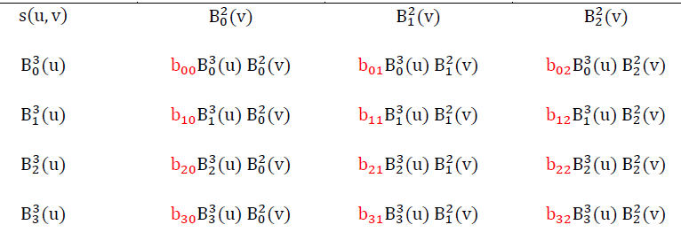
• Dividing s with $x(u, v), y(u, v), z(u, v)$

\[x(u, v) = \sum_{i=0}^m \sum _{j=0}^n b_{ij}^x B_i^m(u) B_j^n(v)\]

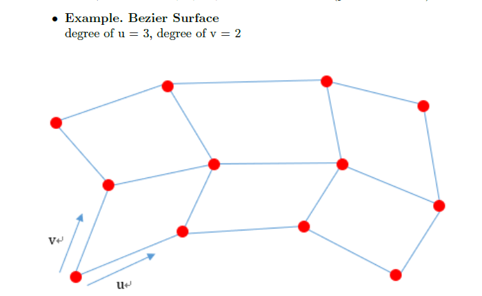
Procedure

1. Connect the control points at the corresponding points to create a control polygon
2. Create a Bezier Surface given the control polygon

2. De Castelijau algorithm for Bezier surface

• Two ways to approach : calculate $u$ first or $v$ first
• Example!

• $u$ → $v$ : $(3+2+1) \times 3 + (2+1) \times 1=21$
• $v $ → $u$ : $(2+1)\times 4 + (3+2+1) \times 1 = 18$
• To reduce the amout of computation, calculating parameters with a small degree first.

3. Convert monomial basis function to Bezier basis function for a surface

• Example !
• Consider $f(u, v) = 1+ 2u - u^2 +4v-2uv +2u^2v$
• degree of $u$ : 2, degree of $v$ : 1

\[\begin{aligned}f(u, v) =& \sum_{i=0}^2 \sum_{j=0}^1 b_{ij} B_i^2(u) B_j^1(v) \\=& \sum_{i=0}^2 \sum_{j=0}^1 b_{ij} {2 \choose i}(1-u)^{2-i}u^i {1\choose j}(1-v)^{1-j}v^j \end{aligned}\]

• Differentiating both sides with respect to $u$ and $v$ are always valid. Figure each coefficient with this way, with substituting $u=0, v=0$ (identity)

Drawing a graph of a Bezier surface function

\[\begin{bmatrix} u \\ v \\f(u, v) \end{bmatrix}\]

• Example (continued)

\[\begin{bmatrix} u \\ v \\f(u, v) \end{bmatrix} = \begin{bmatrix} 0/2B_0^2(u) + 1/2 B_1^2(u) + 2/2 B_2^2(u) \\ 0/1 B_0^1(v) + 1/1B_1^1(v) \\\sum\sum b_{ij}B_i^2(u)B_j^1(v) \end{bmatrix}\]

• with using sum-to-one property,

\[\begin{bmatrix} u \\ v \\f(u, v) \end{bmatrix} = [B_0^m(u) \cdots B_m^m(u)] \begin{bmatrix}{\bf b_{00} } & \cdots & {\bf b_{0n} } \\ \vdots & \ddots & \vdots \\ {\bf b_{m0} } & \cdots & {\bf b_{mn} } \end{bmatrix}\begin{bmatrix}B_0^n(v) \\ B_n^n(v)\end{bmatrix}\]

where

\[{\bf b_{ij}} = \begin{bmatrix}{i \over n} \\ {j \over m} \\ b_{ij}\end{bmatrix} = \begin{bmatrix}u \\ v \\f(u, v)\end{bmatrix}\]

4. Local support

B-spline (Basis spline)

• Non-negativity
• Sum-to-one property
• Local support
• Same size of support [$u_i , u_{i+p+1}$)

Local support

• support : parameter area where the function value is not zero
• Local support : Parameter region where the function value is not 0 is local
• Global support : lots of nonzero..
• Local support is numerically stable and faster computation speed

5. Interpolation and Approximation

• Example !
• Residual $e_i = y_i - f(x_i)$
• Total residual is squared sum of residual

\[\varepsilon(a, b) = e_1^2+e_2^2+e_3^2 = ||A\hat x -b || ^2\]

• Each term $a, b$ is determining by finding value that minimizes total residual function : ${\partial \varepsilon(a, b) \over \partial a}= 0, {\partial \varepsilon(a, b) \over \partial b}= 0$

Residual vs error

• error : $\vert\vert \hat x - x\vert\vert$
• residual : $\vert\vert A\hat x - b \vert\vert$
• if error is zero ($x=\hat x$) → $A\hat x = b$ (sufficient)
• if residual ($\vert\vert A\hat x -b \vert\vert = 0$) → $A\hat x = b$ (not always true, necessary)

6. Tangent vector

• Consider a bezier curve with degree $n$

\[{\bf x} (t) = \sum_{i=0}^n b_i B_i^n (t)\] \[{d\over dt}B_i^n (t) = n[B_{i-1}^{n-1}(t)-B_{i}^{n-1}(t)]\]

• Degree of Bernstein basis decreased by 1, difference btw $i-1$ and $i$, $n$ omitted (recall differentiation of power series)

\[{\bf \dot x}(t) = {d\over dt} {\bf x}(t)= n\sum_{i=0}^{n-1}\Delta b_i B_i^{n-1}(t) \ \Delta b_i = b_{i+1}-b_i\]

• Also $n$ omitted with decreasing degree of bernstein basis, index moved $(0, n)$ to $(0, n-1)$, note that $\Delta b_i = b_{i+1}-b_i$

Geometrical interpretation

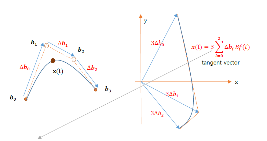
• Tangent vector is also a Bernstein with decreased degree, each control point is $n$ (original degree) times vector of original adjacent control points
• If the term satisfies (sum-to-zero) property : it is vector, (sum-to-one) property : it is point (on curve)

Application on higher order derivatives

\[{\bf x}''(t) = n(n-1) \sum_{i=0}^{n-2} \Delta^2b_i B_i^{n-2}(t)\]

where $\Delta^2b_i = \Delta b_{i+1}-\Delta b_i = (b_{i+2} - 2b_{i+1} + b_i)$

each coefficient is ${n \choose m}(-1)^{n}$

Global tangent vector application

• consider a global spline $u\in[a, b]$

\[{\bf x}(u) = \sum_{i=0}^n b_i B_i^n (u)\] \[{\bf x}'(u) = {d\over du} {\bf x} (u) = {d{\bf x}(t) \over dt} \cdot {dt \over du} = {\bf x}'(t) \cdot {1\over {b-a}}\]

because, $t= {u-a\over b-a}$ by parameterization, ${dt\over du} = {1\over b-a}$

\[={1\over b-a} n\sum_{i=0}^{n-1}\Delta b_i B_i^{n-1}(t), \ t\in[0, 1]\]