[신호 및 시스템] Lec 04, 05 - Convolution, Impulse response

Precaution

본 게시글은 서울대학교 박성준 교수님의 신호 및 시스템 (26 Spring) 강의록입니다.

Definition of convolution

• DT

\[y[n] = x[n] * h[n] = \sum_{m=-\infty}^\infty x[m]h[n-m]\]

• CT

\[y(t) = x(t) * h(t) = \int_{-\infty}^\infty x(\tau) h(t-\tau) d\tau\]

• An arbitary LTI system can be obtained as the convolution of the input signal and the system’s impulse response
• General step-by-step calculation (Example on DT)
  1. given $n$
  2. Flip $h[k] \rightarrow h[-k]$
  3. Shift $h[-k] \rightarrow h[n-k]$
  4. Sum $\sum x[k]h[n-k]$ in respect to $k$

Convolution with impulse function

• $h[n] = \delta [n-n_0]$
• $y[n] = \sum_{-\infty}^\infty h[n-k]x[k] = \sum x[k]\delta[n-n_0-k]$
• $y[n]=x[n-n_0]$

Impulse Response

• Impulse response of system is a output when inputting $\delta(t)$ impulse function

Impulse response in LTI system (DT)

\[\begin{aligned}x[n] &= \cdots + x[-1]\delta[n+1] + x[0]\delta[n] + x[1]\delta[n-1] + \cdots \\ &= \sum_{k=-\infty}^\infty x[k]\delta[n-k] \end{aligned}\]

• Sampling property of impulse function
• From linearity :

\[\begin{aligned}y[n] &= \cdots + x[-1]H\{\delta[n+1]\} + x[0]H\{\delta[n]\} + x[1]H\{\delta[n-1]\} + \cdots \\ &= \sum_{k=-\infty}^\infty x[k]H\{\delta[n-k]\} \end{aligned}\]

• From time invariance :

\[\sum_{k=-\infty}^\infty x[k]H\{\delta[n-k]\} = \sum_{k=-\infty}^\infty x[k]h[n-k] = x[n]*h[n]\]

• Interpretation : for an arbitary input $x[n]$ and an LTI system with an impulse response $h[n]$, given output $y[n]$ is the convoluation of the input and the impulse response

Impulse response of LTI system (CT)

• say $\delta_{\Delta }(t) = \begin{cases}{1\over \Delta}, & 0\leq t < \Delta \ 0, & \text{else}\end{cases}$
• $H{\delta_{\Delta}(t)} = \hat h_{\Delta}(t)$

\[\hat x(t) = \sum_{-\infty}^\infty x(k\Delta) \delta_{\Delta}(t-k\Delta)\Delta\]

• Simular to sampling property of delta function, by linearity

\[\hat y(t) = \sum_{k=-\infty}^\infty x(k\Delta) h_{\Delta}(t-k\Delta)\Delta\]

• (by time invariance)

\[\begin{aligned}y(t) = \lim_{\Delta \to 0} \hat y(t) &= \lim_{\Delta \to 0} \sum_{k=-\infty}^\infty x(k\Delta) h_{\Delta}(t-k\Delta)\Delta \\ &= \int_{-\infty}^\infty x(\tau)h(t-\tau) d\tau\end{aligned}\]

Linear Constant-Coefficient Differential Equation

• General form :

\[\lbrack a_N{d^N\over dt^N} + a_{N-1}{d^{N-1}\over dt^{N-1}}+ \cdots + a_0 \rbrack y(t) = \lbrack b_M{d^M\over dt^N} + b_{N-1}{d^{N-1}\over dt^{N-1}}+ \cdots + b_0 \rbrack x(t)\]

that is …

\[\sum_{k=0}^N a_ky^{(k)}(t) = \sum_{l=0}^M b_kx^{(l)}(t)\]

• Particular solution (forced response)
• $y(t) = y_p(t), x(t) = x(t)$
• Homogeneous solution (natural response)
• $\sum_{k=0}^N a_k {d^k \over dt^k}y_h(t)=0$
• Overall solution : $y(t) = y_p(t) + y_h(t)$
• Since LCCDE is an LTI system, once we find $h(t)$ ( the particular solution for impulse input) → then $y(t) = x(t) * h(t) $for an arbitary input $x(t)$

LCCDE : Homogeneous solution

\[\sum_{k=0}^N a_k {d^k \over dt^k}y_h(t)=0\]

• try $y_h(t) = Ae^{st}$

\[A\sum_{k=0}^N a_k s^ke^{st}=0, \sum_{k=0}^N a_ks^k=0\]

• $y_h(t) = Ae^{st}$ where $s$ is a solution for $\sum_{k=0}^N a_ks^k=0$ and $A$ can be any value

LCCDE : Particular solution

• Particular solution for input $e^{st}$
• Lets’s try $y_p(t) = Ae^{st}$ again.

\[A\sum_{k=0}^N a_ks^ke^{st} = \sum_{l=0}^N b_ls^le^{st}\] \[A = {\sum _{l=0}^N b_ls^l \over \sum _{k=0}^N a_k s^k}\]

and $y_p(t) = Ae^{st}$ is the particular solution of the ODE

LCCDE and LTI system

• We know this system is LTI

$x(t) = \sum_o \alpha_o e^{s_o t}$

\[y(t) = \sum_o A_o \alpha_o e^{s_ot}\]

where

\[A_o = {\sum _{l=0}^N b_ls_o^l \over \sum _{k=0}^N a_k s_o^k}\]

DT : Linear constant-coefficient difference equation

\[a_N y[n-N] + \cdots a_0 y[n] = b_Mx[n-M] + \cdots b_0 x[n]\] \[\sum_{k=0}^N a_k y[n-k] = \sum_{l=0}^M b_l x[n-l]\]

we can put every term except for $y[n]$ at RHS

• Let $x[n] = \delta[n]$

\[y[n] = -\sum_{k=1}^N {a_k\over a_0}y[n-k] + \sum_{l=0}^M {b_l\over a_0}\delta[n-l]\]

Case I : $a_k=0 (k>0)$

\[y[n] = \sum_{l=0}^M {b_l \over a_0} \delta [n-l], h[n] = \begin{cases} {b_n \over a_0}, & 0 \leq n \leq N \\ 0, & \text{otherwise} \end{cases}\]

• So-called FIR(FInite Impulse response)

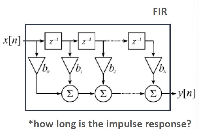
• The impulse response lasts for only $0\leq n\leq M$
• Feedforward : non-recursive

Case II : (general)

\[y[n] = {1\over a_0}\bigg[\sum_{l=0}^M b_l \delta[n-l] - \sum_{k=1}^N a_k y[n-k]\bigg]\]

• The impulse response is not explicitly obtained.
• Infinite Impulse response ( the right summation term works as feedback)

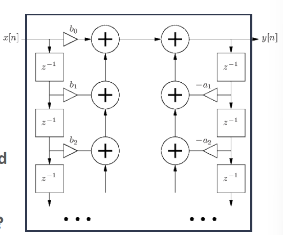
• Feedback (recursive)
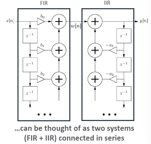
• Can be thought of as two systems (FIR + IIR) connected in series

Can IIR system have finite length output?

• Suppose the system has finite length output, which means

\[\exists n_0 \text{ such that } y[n_0]\neq 0, y[n]=0 \text{ for }n>n_0\]

• Without loosing generality, we can set $a_0=1$
• Construct matrix, we can empty out Lower trianguler term, every pivot is nonzero → matrix A is invertible.
• for invertible matrix $A$, $Ax=0 \Leftrightarrow x=0$
• It contradicts the definition of IIR ($a_i=0$)
• → Any DT system with recursive path cannot have finite length output