[신호 및 시스템] Lec 02 - Properties of signal

Precaution

본 게시글은 서울대학교 박성준 교수님의 신호 및 시스템 (26 Spring) 강의록입니다.

Even signals vs odd signals

• Even signal : $x (t) = x(-t), x[n]=x[-n]$
• Odd signal : $x(t)=-x(-t), x[n]=-x[-n]$
• Note : An arbitary signal can be decomposed into a sum of these two

\[\begin{aligned}x(t) &= x_e(t) + x_o(t) \\ &=0.5(x(t)+x(-t)) + 0.5 (x(t) - x(-t))\end{aligned}\]

Periodic signal

• CT : $x(t) = x(t+T)$ for all t
• DT : $x[n]=x[n+N]$ for all n

Sinusoidal signals

• CT : $x(t) = A\cos {\omega t + \theta}$
• DT : $x[n] = A\cos{[\Omega n + \theta]}$
• In case of CT, sinusoidal signals are always periodic with period $T$
• Otherwise, in case of DT, sinusoidal signals are not always periodic
  • $x[n]=x[n+N]$
  • $A\cos[\Omega n+\theta] = A\cos[\Omega(n+N)+\theta]$
  • Periodic if $\Omega N = 2\pi n$ where $N, m$ integers

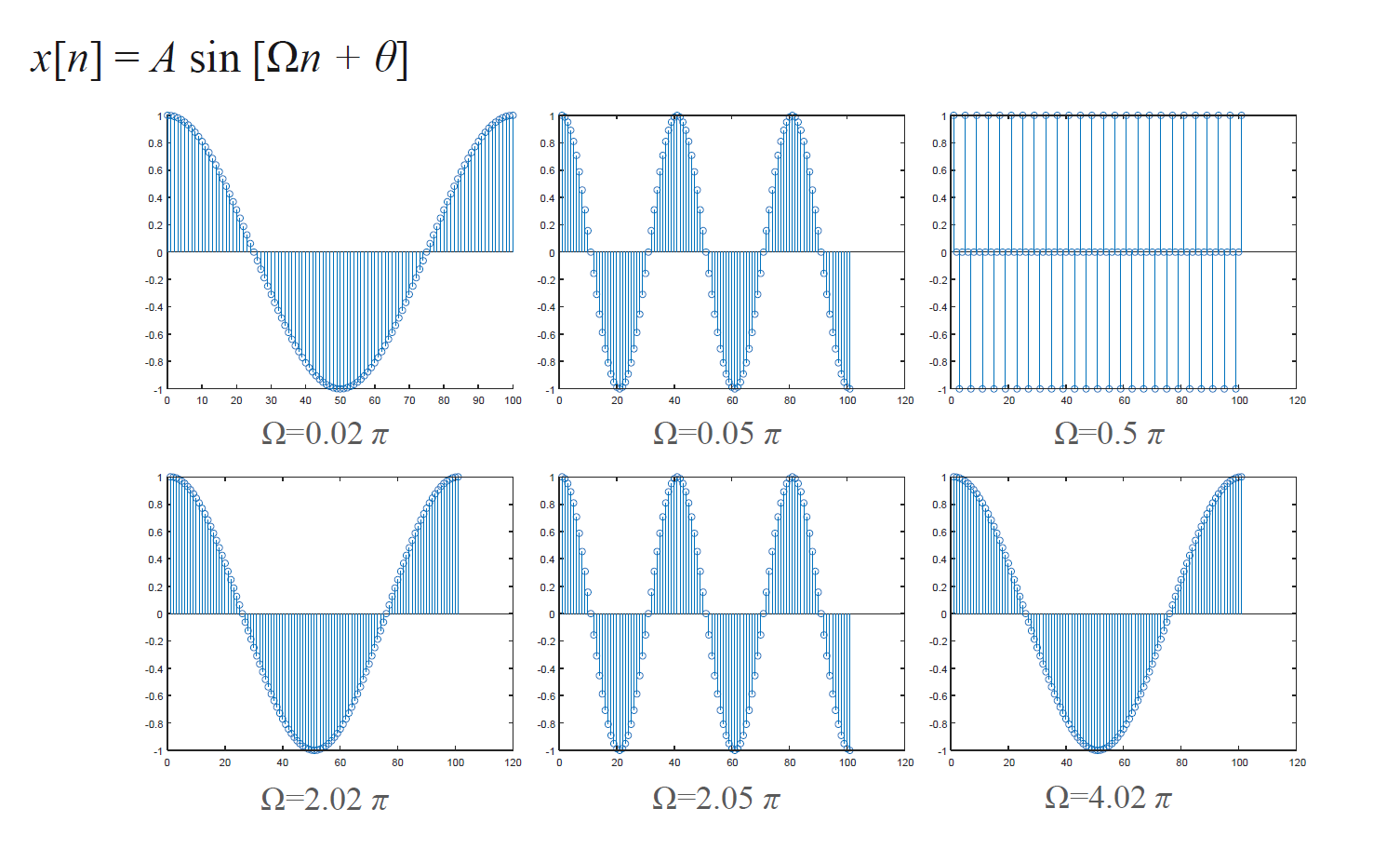
• As $\Omega$ increases, the samples miss the faster oscilllatory behavior

Complex exponential signals

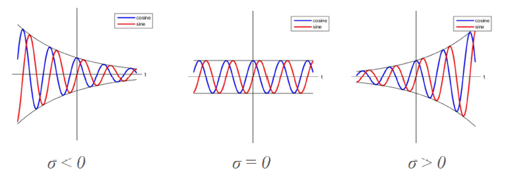
• CT : $x(t) = Ce^{st} = Ce^{(\sigma+j\omega) t}$
• DT : $x[n] = Ce^{sn} = Ce^{(\sigma+j\omega) n}$
• By euler’s equation, complex exponential and sinusoidals can be thought of as almost the same thing
• $\cos \theta = Re{e^{j\theta}}={e^{j\theta} + e^{-j\theta}\over 2}$
• $\sin \theta = Im{e^{j\theta}}={e^{j\theta} - e^{-j\theta}\over 2j}$
• $x(t) = Ce^{(\sigma + j\omega)t} = Ce^{\sigma t}(\cos \omega t + j \sin \omega t)$

• Same things applied on DT

Periodicity of complex exponential term

• CT : $x(t) = x(t+T)$
• $e^{j\omega t} = e^{j\omega (t+T)}$
• Period $e^{j\omega T} = 1 \Rightarrow T={2\pi \over \omega}$
• DT : $x[n] = x[n+N]$
• $e^{j \omega n} = e^{j \omega (n+N)}$
• Period $e^{j\omega N} = 1 \Rightarrow N=m{2\pi \over \omega} \in \N$

Unit step function

• CT : $u(t) = \begin{cases}1, & t\geq 0 \ 0, & t<0\end{cases}$
• DT : $u(n) = \begin{cases}1, & n\geq 0 \ 0, & n<0\end{cases}$

Unit impulse

• DT : $ \delta[n] = u[n]-u[n-1]$ ( Kronecker delta)
• $\delta[n] = \begin{cases} 1, & n=0 \ 0, & n\neq 0 \end{cases}$

\[u[n] = \sum_{m=-\infty}^n \delta[m]\]

• while $m<0$, $\delta[\cdot]$ is zero for all $m$. $\delta[m]$ is $1$ only for positive $m$ ($0 \sim n$)
• $m=-\infty$ for considering negative $n$
• DT : $\delta (t) = \lim_{\Delta\to 0}\delta_{\Delta}(t)$
• $\delta(t) = \begin{cases}+\infty, & t=0 \ 0, & t \neq 0\end{cases}$

\[\int_{-\infty}^\infty \delta(t) dt = 1\] \[u(t) = \int_{-\infty}^t\delta(\tau)d\tau\]

Sampling as product with unit impulse

\[\begin{aligned} x[n]\delta[n-n_0] = x[n_0]\delta[n-n_0] \\ \sum_{n=-\infty}^\infty x[n]\delta[n-n_0] = x[n_0] \end{aligned}\]

• Sample at $n=n_0$ with $\delta[n-n_0]$

Operation on signals

• Amplitude scaling : $H : x(t) \rightarrow y(t) = Kx(t)$
• Time translation : $H : x(t) \rightarrow y(t) = x(t-t_0)$
  • $t\leftarrow t-t_0$
• Time scaling : $H : x(t) \rightarrow y(t) = x(t/a)$
  • $t\leftarrow t/a$
  • $a>1$ : stratch the time domain
  • $0<a<1$ : shrink the time domain
  • $a=-1$ : time reverse
• The order of operation matters.