[신호 및 시스템] Lec 08, 09 - Continuous/Discrete Time Fourier Series

Precaution

본 게시글은 서울대학교 박성준 교수님의 신호 및 시스템 (26 Spring) 강의록입니다.

Periodic signals and harmonics

• consider $x(t)$ with fundamental period $T$ (Fundamental frequency $\omega _0 = {2\pi \over T}$)
• Harmonics : complex exponentials (or sinusoids) whose frequencies are integer multiples of the fundamental frequency
• $\phi_{c, k}(t) = e^{jk\omega_0 t} = e^{jk{2\pi\over T} t}, k=0, \pm 1, \pm 2 , \cdots$
• Harmonic representations : Periodic signals can be represented as a sum of harmonics

\[x(t) = \sum_{k=-\infty}^\infty a_k e^{jk\omega_0 t} = \sum_{k=-\infty}^\infty a_k e^{jk{2\pi\over T} t}\]

Fourier series representation

• Mathematical property for finding $a_k$

\[\int_{t_0}^{t_0+T}e^{jk\omega_0 t}dt = \int_T e^{jk\omega_0 t} dt = \begin{cases}0, & k\neq 0 \\ T, & k=0\end{cases} = T\delta[k]\] \[x(t) = \sum_{k=-\infty}^{\infty} a_k e^{j k \omega_0 t}\] \[\int_T x(t)e^{-j l \omega_0 t} \, dt=\int_T \sum_{k=-\infty}^{\infty} a_k e^{j k \omega_0 t} e^{-j l \omega_0 t} \, dt\] \[= \sum_{k=-\infty}^{\infty} a_k \int_T e^{j (k-l)\omega_0 t} \, dt= \sum_{k=-\infty}^{\infty} a_k T \delta[k-l]= T a_l\] \[a_k = \frac{1}{T} \int_T x(t)e^{-j k \omega_0 t} \, dt= \frac{1}{T} \int_T x(t)e^{-j k \frac{2\pi}{T} t} \, dt\]

CT Fourier Series

• Analysis

\[a_k = \frac{1}{T} \int_T x(t)e^{-j k \frac{2\pi}{T} t}\,dt\]

• Synthesis

\[x(t) = \sum_{k=-\infty}^{\infty} a_k e^{j k \frac{2\pi}{T} t}\]

Dirichlet conditions for pointwise convergence

• There is no energy in the difference $\int_T \vert e(t)\vert^2 dt = 0$ where $e(t) = x(t) - \sum_{k=-\infty}^{\infty} a_k e^{j k \frac{2\pi}{T} t}$
• if $\int_T \vert x(t)\vert^2 dt < \infty$ ($x(t)$ has finite energy per period)
• Condition 1 : $x(t)$ is absolutely integrable over one period, i.e.
• Condition 2 : In a finite time interval, $x(t)$ has a finite number of maxima and minima.
  • $x(t) = \sin (2\pi /t)$ : Violates condition 2
• Condition 3 : $x(t)$ has only a finite number of discontinuities

\[\sum_{k=-\infty}^{\infty} a_k e^{j k \frac{2\pi}{T} t}=\frac{1}{2}\left(x(t^-) + x(t^+)\right)\]

• The fourier series : “midpoint” at points of discontinuity

Fourier Series

Mean value

\[a_k = \frac{1}{T} \int_0^T x(t)e^{-j k \omega_0 t}\,dt \Rightarrow_{k=0} a_0 = \frac{1}{T} \int_0^T x(t)\,dt\]

Constant ↔ Impulse

• Scalar constant
• $A \xLeftrightarrow{\mathrm{FS}} A\delta[k]$

\[a_k = \frac{1}{T} \int_0^T A e^{-j k \omega_0 t}\,dt= A \frac{e^{-j k \omega_0 T} - 1}{-j k \omega_0 T}=\begin{cases}A, & k = 0 \\0, & k \ne 0\end{cases} =A\delta[k]\]

• Periodic impulses
• $\sum_{n=-\infty}^{\infty} \delta(t - nT)\xLeftrightarrow{\mathrm{FS}}\frac{1}{T}$

\[a_k = \frac{1}{T} \int_{nT - \frac{T}{2}}^{nT + \frac{T}{2}} \delta(t - nT)e^{-j k \omega_0 t}\,dt= \frac{1}{T} e^{-j k n \omega_0 T}= \frac{1}{T}\]

Time & Frequency Shift

• Time shift

\[\tilde{x}_T(t - t_0)\xLeftrightarrow{\mathrm{FS}}a_k e^{-j k \omega_0 t_0}\] \[\tilde{x}_T(t - t_0)= \sum_{k=-\infty}^{\infty} a_k e^{j k \omega_0 (t - t_0)}= \sum_{k=-\infty}^{\infty} a_k e^{-j k \omega_0 t_0} e^{j k \omega_0 t}\]

→ $t \leftarrow t-t_0$ : Follows the original sign

• Frequency shift

\[\tilde{x}_T(t)e^{j k_0 \omega_0 t}\xLeftrightarrow{\mathrm{FS}}a_{k - k_0}\] \[a'_k= \frac{1}{T} \int_0^T \tilde{x}_T(t)e^{j k_0 \omega_0 t} e^{-j k \omega_0 t}\,dt= \frac{1}{T} \int_0^T \tilde{x}_T(t)e^{-j (k - k_0)\omega_0 t}\,dt= a_{k - k_0}\]

→ $k \leftarrow k-k_0$ : reverses the original sign

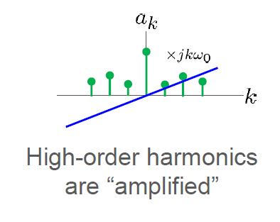
Differentiation & integration

• Differentiation

\[\frac{d}{dt}\tilde{x}_T(t)\xLeftrightarrow{\mathrm{FS}}j k \omega_0 a_k\] \[\frac{d}{dt}\left(\sum_{k=-\infty}^{\infty} a_k e^{j k \omega_0 t}\right)= j k \omega_0 \sum_{k=-\infty}^{\infty} a_k e^{j k \omega_0 t}\]

• $jk\omega_0$ omits.
• Geometrical Interpretation : Higher-order harmonics are amplified

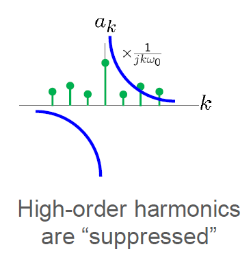
• Integration

\[\int_{-\infty}^{t} \tilde{x}_T(\tau)\,d\tau\xLeftrightarrow{\mathrm{FS}}\frac{1}{j k \omega_0} a_k\] \[\sum_{k=-\infty}^{\infty} a_k \int_{-\infty}^{t} e^{j k \omega_0 \tau}\,d\tau= \sum_{k=-\infty}^{\infty} \left(\frac{1}{j k \omega_0} a_k\right) e^{j k \omega_0 t}\]

• $1/jk\omega_0$ omits.
• Geometrical interpretation : Higher-order harmonics are suppresed

Flip

\[\tilde{x}_T(-t)\xLeftrightarrow{\mathrm{FS}}a_{-k}\quad (= a_k^* \text{ for real } \tilde{x}_T(t))\] \[\tilde{x}_T(-t)= \sum_{k=-\infty}^{\infty} a_k e^{-j k \omega_0 t}= \sum_{k=-\infty}^{\infty} a_{-k} e^{j k \omega_0 t}\]

• Fourier coefficient also flipped
• Application to even, odd function :
  • Even function $\tilde{x}T(-t) = \tilde{x}_T(t) \xLeftrightarrow{\mathrm{FS}} a{-k} = a_k$
  • Odd function $\tilde{x}T(-t) = -\tilde{x}_T(t) \xLeftrightarrow{\mathrm{FS}} a{-k} = -a_k$
  • Even → Even, Odd → Odd : Even odd property still remains

Time scaling

\[\tilde{x}_T(\alpha t)\xLeftrightarrow{\mathrm{FS}}a_k\quad (\omega_0 \rightarrow \alpha \omega_0)\] \[\tilde{x}_T(\alpha t)= \sum_{k=-\infty}^{\infty} a_k e^{j k \omega_0 \alpha t}= \sum_{k=-\infty}^{\infty} a_k e^{j k (\alpha \omega_0) t}\]

• For coefficient $\alpha$ affects the frequency, not the coefficient directly
• for $\alpha>1$, shrinking the original function works as multiplication of same factor to frequency

Conjugate symmetric

• If $x(t)$ is real, then $a_{-k} = a_k^$ and $a_k = a_{-k}^$

\[\begin{aligned} x(t) &= \sum_{k=-\infty}^{\infty} a_k e^{j k \omega_0 t}= x^*(t)= \sum_{k=-\infty}^{\infty} a_k^* e^{-j k \omega_0 t} \\ &= \sum_{l=-\infty}^{\infty} a_{-l}^* e^{j l \omega_0 t} = \sum_{k=-\infty}^{\infty} a_{-k}^* e^{j k \omega_0 t}\end{aligned}\] \[\therefore a_{-k}^* = a_k\]

• Which means, the real part of $a_k$ of real function is even, while odd part of $a_k $ is odd.

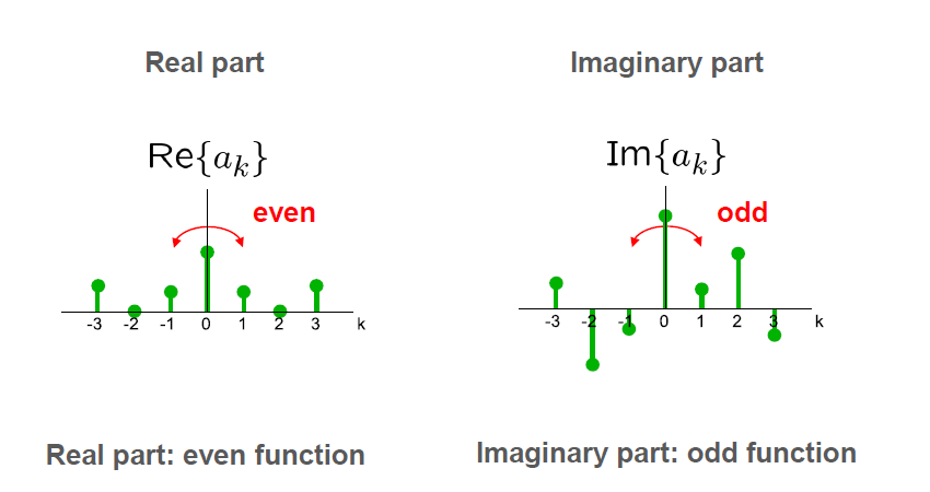
• Interpretation as a complex exponential function, in terms of magnitude → even function, phase → odd function

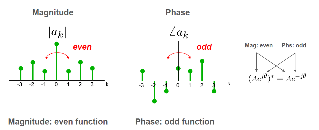
Complex conjugate : Conclusion

• $x(t)$ is real, even → $a_k$ are conjugate even and even → $a_k $ are real, even.
• $x(t)$ is real, odd → $a_k$ are conjugate even and odd → $a_k$ are pure imaginary, odd

Multiplication

$\tilde{x}_T(t)\xLeftrightarrow{\mathrm{FS}}a_k,\tilde{y}_T(t)\xLeftrightarrow{\mathrm{FS}}b_k$

\[\tilde{x}_T(t)\tilde{y}_T(t)\xLeftrightarrow{\mathrm{FS}}\sum_{m=-\infty}^{\infty} a_m b_{k-m}\]

• Multiplication → convolution

\[\begin{aligned}\tilde{x}_T(t)\tilde{y}_T(t)&= \left(\sum_{m=-\infty}^{\infty} a_m e^{j m \omega_0 t}\right)   \left(\sum_{n=-\infty}^{\infty} b_n e^{j n \omega_0 t}\right) \\&= \sum_{m=-\infty}^{\infty} \sum_{n=-\infty}^{\infty} a_m b_n e^{j (m+n)\omega_0 t} \\&= \sum_{m=-\infty}^{\infty} \sum_{k=-\infty}^{\infty} a_m b_{k-m} e^{j k \omega_0 t} \\&= \sum_{k=-\infty}^{\infty} \left(\sum_{m=-\infty}^{\infty} a_m b_{k-m}\right) e^{j k \omega_0 t}\end{aligned}\]

Convolution

$\tilde{x}_T(t)\xLeftrightarrow{\mathrm{FS}}a_k, \tilde{y}_T(t)\xLeftrightarrow{\mathrm{FS}}b_k$

\[\tilde{x}_T(t) * \tilde{y}_T(t)\xLeftrightarrow{\mathrm{FS}}T a_k b_k\] \[\begin{aligned} \tilde{x}_T(t) * \tilde{y}_T(t) &= \int_0^T \left[\sum_{m=-\infty}^{\infty} a_m e^{j m \omega_0 \tau} \sum_{n=-\infty}^{\infty} b_n e^{j n \omega_0 (t-\tau)}\right] d\tau \\ &= \sum_{m=-\infty}^{\infty} \sum_{n=-\infty}^{\infty} a_m b_n \left(\int_0^T e^{j (m-n)\omega_0 \tau} d\tau\right) e^{j n \omega_0 t} \\ &= \sum_{m=-\infty}^{\infty} \sum_{n=-\infty}^{\infty} a_m b_n (T\delta_{mn}) e^{j n \omega_0 t} \\ &= \sum_{n=-\infty}^{\infty} T a_n b_n e^{j n \omega_0 t} \end{aligned}\]

• by the property of Fourier series (intergrate over one period) → $T$ omits

Parseval’s relation

\[\frac{1}{T}\int_T |\tilde{x}_T(t)|^2 dt=\sum_{k=-\infty}^{\infty} |a_k|^2\]

• Average power over one period = Total squared sum of fourier series coefficient

\[\frac{1}{T}\int_T |\tilde{x}_T(t)|^2 dt= \sum_{k=-\infty}^{\infty} \frac{1}{T}\int_T |a_k e^{j k \omega_0 t}|^2 dt = \sum_{k=-\infty}^{\infty} |a_k|^2\]

Example : periodic rectangular function

$\mathrm{rect}(t) =\begin{cases}1, &

t

\le 0.5 \0, &

t

> 0.5\end{cases}$

\[\begin{aligned}a_k&= \frac{1}{T}\int_{-L/2}^{L/2} e^{-j k \omega_0 t}\,dt \\&= -\frac{1}{j k \omega_0 T} \left[ e^{-j k \omega_0 t} \right]_{-L/2}^{L/2} \\&= -\frac{1}{j k \omega_0 T} \left( e^{-j k \omega_0 \frac{L}{2}} - e^{j k \omega_0 \frac{L}{2}} \right) \\&= -\frac{1}{j k \omega_0 T} \left( -2j \sin\left(\frac{k \omega_0 L}{2}\right) \right) \\&= \frac{1}{k\pi} \sin\left(\frac{k\pi L}{T}\right) \\&= \frac{L}{T} \frac{\sin\left(\frac{k\pi L}{T}\right)}{\frac{k\pi L}{T}} = {L\over T}\text{sinc}({k\pi L \over T})\end{aligned}\]

DT Fourier Series

• Analysis

\[a_k = {1\over N} \sum_{<N>} x[n] e^{-j{2\pi k n \over N}}\]

• Synthesis

\[x[n] = \sum_{k=<N>} a_ke^{j{2\pi k n \over N}}\]

Linearity, time-frequency shift

• Time shift

\[\tilde x_N[n-n_0] \xLeftrightarrow{\mathrm{FS}} a_k e^{-jk{2\pi \over N} n_0}\]

• Frequency shift

\[\tilde x_N[n] e^{jk_0 {2\pi\over n} n} \xLeftrightarrow{\mathrm{FS}} a_{k-k_0}\]

Convolution, multiplication

• (Periodic) Convolution

$\tilde{x}_1[n]\xLeftrightarrow{\mathrm{FS}}a_k,\tilde{x}_2[n]\xLeftrightarrow{\mathrm{FS}}b_k$

\[\tilde{z}_N[n]= \sum_{k=\langle N \rangle} \tilde{x}_N[k]\tilde{y}_N[n-k]\xLeftrightarrow{\mathrm{FS}}c_k = N a_k b_k\] \[\tilde{z}_N[n]= \tilde{x}_N[n]\tilde{y}_N[n]\xLeftrightarrow{\mathrm{FS}}c_k = \sum_{l=\langle N \rangle} a_l b_{k-l}\]

• In case of convolution, $N$ omits

Difference, running sum

• Difference

\[\tilde{x}_N[n] - \tilde{x}_N[n-1]\xLeftrightarrow{\mathrm{FS}}\left(1 - e^{-j k \frac{2\pi}{N}}\right)a_k\]

• Just summation of original FS + time shift FS
• Running sum

\[\sum_{k=-\infty}^{n} \tilde{x}_N[k]\xLeftrightarrow{\mathrm{FS}}\frac{1}{1 - e^{-j k \frac{2\pi}{N}}} a_k\]

• Work as infitnite sum of series with $r = e^{-jk\Omega_0}$

Time-scaling

\[\tilde{x}_{mN}[n] =\begin{cases}\tilde{x}_N[n/m], & \text{if } n/m \text{ is integer} \\0, & \text{otherwise}\end{cases}\xLeftrightarrow{\mathrm{FS}}\frac{1}{m} a_k\]

• Works conversely : for CT $x(t) \rightarrow x(\alpha t)$ but in case of DT $x_N[n] \rightarrow x_{mN}[n]=x_N[n/m]$
• for $m>1$, stretches the signal, and fills the hole with zero

Conjugate symmetric

• If $x_N[n]$ is real, then $a_{-k} = a_k^$ and $a_k = a_{-k}^$

\[\tilde x_N[n]^* \xLeftrightarrow{\mathrm{FS}} a_{-k}^*\]

Parseval’s relation

\[\frac{1}{N} \sum_{k=\langle N \rangle} |\tilde{x}_N[n]|^2=\sum_{k=\langle N \rangle} |a_k|^2\]