[유체] Chap 11. Basics of Viscous Flow

Chap 11. Basics of Viscous Flow

11.1 Definitions

\[\tau = \mu {\partial u \over \partial y}\]

• If $\mu $ is constant, it is Newtoninan fluid
• Newtonian fluid : a fluid in which the viscous str ess are linearly correlated to the local strain rate
• In einstein notaiton

\[\tau_{ij} = \mu({\partial u_i \over \partial x_j} + {\partial u_j \over \partial x_i}) (i\neq j)\]

Stress tensor

\[\sigma _{ij} = -p\delta_{ij} + \tau_{ij}\]

• in Vector Notation

\[\begin{bmatrix} \ \\ \sigma_{ij} \\ \ \end{bmatrix} = \begin{bmatrix} -p & \tau_{12} & \tau_{13} \\ \tau_{21} & -p & \tau_{23} \\ \tau_{31} & \tau_{32} & -p \end{bmatrix}\]

• $\mu$ : dynamic viscosity, ($kg/m\cdot s$)
• $\nu$ : kinematic viscosity, ($m^2 /s$)

11.2 Key nondimensional Parameter in Viscous Flow

\[F = ({\vec \sigma \cdot \vec n})ds\]

• Reynolds Number

\[Re = {UL\over \nu}\]

• Ratio between inertia force and viscous force
• Low Reynolds number : Viscosity dominent(Laminar) , High Re : Inertia dominent (Turbulant)
• Drag coefficient

\[C_D = {F_D\over {1\over 2} \rho SU^2}\]

• $S$ : in general, projected area, in ship, Wetted Surface Area
• Drag consists of Friction al Drag($C_f, \tau_{ij}$) + Pressure drag ($p\delta_{ij}$)

Kinematic Condition

• No-penetration condition : $u_n = 0$ or $u_n = U\cdot \vec n$
• No-slip condition

\[u_t = U\cdot \vec t\]

• Free slip condition on potential flow ($u_t \neq 0$) no necessary to be zero
• Flow seperation happens on ${\partial u \over \partial y} = 0$

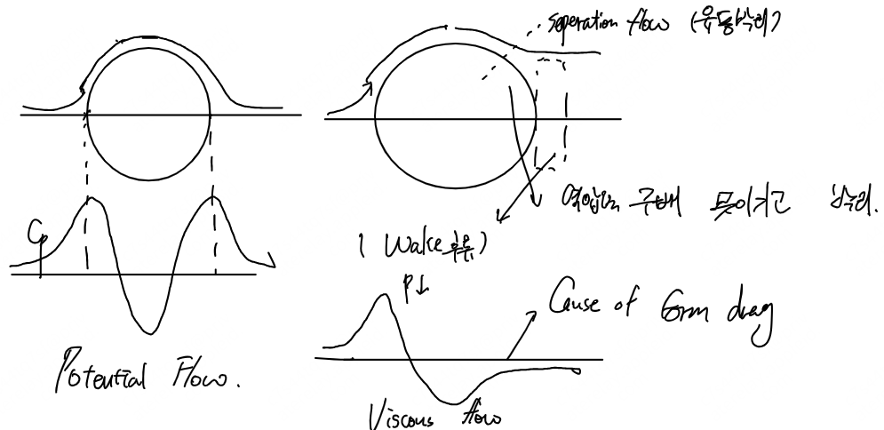
• $C_p = {P \over {1\over 2 } \rho u^2}$

Cylinder (Laminar vs Turbulant)

• All viscous flow : thus seperation always happens

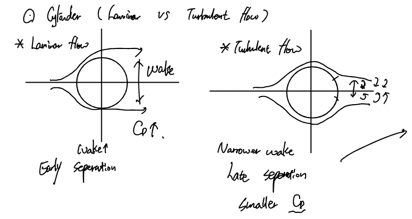
• Reasons of making dimple on golf ball. Turbulance makes late seperation, which causes smaller $C_D$
• Ideal flow : $Re = \infty$ as $\nu \to 0$ → No seperation happens

11.3 Differential Equations for viscous flow

• Remind : Euler equation and its derivation

\[{d\vec u \over dt} = {\partial \vec u \over \partial t} + (\vec u \cdot \nabla ) \vec u = \vec f + {1\over \rho}\nabla \cdot \overline{\overline{\sigma}}\]

and $\sigma_{ij} = -p\delta_{ij} + \tau_{ij}$

\[\nabla \cdot \sigma_{ij} = {\partial \sigma_{ij} \over \partial x_j} = {\partial (-p\delta_{ij})\over \partial x_j}+ \mu {\partial \over \partial x_j} \big({\partial u_i\over \partial x_j} + {\partial u_j \over \partial x_i}\big)\] \[= -\nabla p + \mu\nabla^2 u_i + ({\partial \over \partial x_i})\cancel{({\partial u_j \over \partial x_j})}\]

• In vector Notation

\[\nabla \cdot \overline{\overline{\sigma}} = \nabla \cdot (-pI) + \mu \nabla \cdot (\nabla \vec u)+ \mu \nabla \cdot (\nabla \vec u)^T = -\nabla p + \mu \nabla^2\vec u+ \mu \nabla \cancel{(\nabla \cdot \vec u)}\]

11.4 Examples of Exact solutions of N-S equation

Flow between two plates : Couette flow

Upper plate moves to x-dirextion with constant velocity $U$

Lower plate stays still, gap between two plate is $h$

• BVP
• Boundary condition

$u=U, v=0 $ on $y=h$ (No-slip, no-penetration condition)

$u=0, v=0$ on $y=0$ (Same)

${\partial \over\partial x} (u, v) = 0$ (No velocity profile change in x-direciton, assumption of Couette flow)

Steady flow : ${\partial \over \partial t}(\cdot ) = 0$

• Governing Equations

\[\nabla \cdot \vec u = 0, {\partial u\over \partial x} + {\partial v \over \partial y} = 0\]

⇒ ${\partial v \over \partial y} = 0$, $v(y) = 0 (v(0) = v(h) = 0)$

\[\cancel{\partial u \over \partial t } + u\cancel{\partial u \over \partial x} + \cancel{v{\partial u \over \partial y}} = -{1\over \rho}{\partial p \over \partial x} + \cancel{ \vec f} + \nu \big(\cancel{\partial^2 u \over \partial x^2} + {\partial ^2 u \over \partial y^2}\big)\] \[{\partial p \over \partial x} = \mu {\partial^2 u \over \partial y^2}\] \[\cancel{\partial v \over \partial t } + u\cancel{\partial v \over \partial x} + v\cancel{\partial v \over \partial y} = -{1\over \rho}{\partial p \over \partial y} + \cancel{ \vec f} + \nu \big(\cancel{\partial^2 v \over \partial x^2} + \cancel{\partial ^2 v \over \partial y^2}\big)\] \[{\partial p \over \partial y} = 0\]

• By integration

\[u = {1\over 2\mu}({\partial p \over \partial x})y^2 + C_1 y + C_2\]

Applying Boundary conditions, $C_2 = 0$

\[C_1 h = U-{1\over 2\mu} ({\partial p \over \partial x})h^2\] \[C_1 = {U\over h} - {h\over 2\mu} {\partial p \over \partial x}\] \[\therefore u = {1\over 2\mu} (y-h)y {\partial p \over \partial x} + {U\over h}y\] \[\tau_{xy} = \mu ({\partial u \over \partial y}) = \mu {U\over h}+ {\partial p \over \partial x}(y-{h\over 2})\]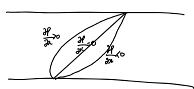

Flow inside a pipe : Poiseulle Flow

• Axi-symmetric flow, $\vec u = (u_x, u_r, u_\theta) = (u_x, 0, 0)$
• Useful Formula in cylenderic / polar coordiante

\[{\partial \hat{e_r}\over \partial \theta } = \hat{e_\theta}, {\partial \hat{e_\theta}\over \partial \theta } = -\hat{e_r}\] \[\nabla = \hat{e_r}{\partial \over \partial r} +\hat{e_\theta}{1\over r}{\partial \over \partial \theta} + \hat{e_x}{\partial \over \partial x}\] \[\nabla \cdot \vec A = {1\over r}{\partial \over \partial r}(rA_r)+ {1\over r} {\partial \over \partial \theta }(A_{\theta}) + {\partial \over \partial x} (A_x)\]

• Continuity eqn

\[{1\over r} \cancel{{\partial \over \partial r}(ru_r)}+ \cancel{{\partial \over \partial x}(u_x)} + {1\over r}\cancel{{\partial \over \partial \theta}(u_\theta) }= 0\]

• N-S eqn

\[\rho \big(\cancel{\partial u \over \partial t}+\cancel{u_r {\partial u \over \partial r}}+ u_\theta {1\over r}\cancel{\partial u \over \partial \theta } + u_x \cancel{\partial u\over \partial x}\big) = \cancel{f_x}- {\partial p \over \partial x} + \mu \big[{1\over r} {\partial \over \partial r}(r{\partial u \over \partial r})+ {1\over r^2 }\cancel{\partial^2 u \over \partial \theta^2} + \cancel{\partial^2 u \over \partial x^2}\big]\] \[{\partial p \over \partial x} = \mu {1\over r} {\partial \over \partial r}(r{\partial u \over \partial r})\]

Integrate,

\[u = {1\over 4\mu}(-{\partial p \over \partial x})(R^2-r^2)\]

• BC : $u=0, r=R, u\neq \infty, r=0$
• Perspective of wall, coordinate is defined

\[\tau = -\mu {\partial u\over \partial r}\vert_{r=R} = {R\over 2}(-{\partial p \over \partial x})\]

11.5 Turbulant flow and RANS equation

• Laminar flow :
  • Layer flow
  • Weak mixing
  • Little fluctuation velocity
  • Viscous-dominant flow Smaller Re
  • Getting Damped motion
• Turbulant flow :
  • Chaotic particle flow
  • Strong mixing
  • Non-ignorable fluction
  • Higher Re
  • Getting growing motion
• Assume that

\[u_i = \overline{u_i} \ + \ u_i'\]

• $\overline{u_i’} = 0$
• $\overline{u_i u_j} = \overline{(\overline{u_i}+u_i’)(\overline{u_j}+u_j’)} = \overline{u_i}\overline{u_j} + \overline{u_i’}\overline{u_j’}$

Continuity equation

\[{\partial u_i \over \partial x_i} = \cancel{\partial \overline{u_i}\over \partial x_i} + {\partial u_i'\over \partial x_i} = 0\]

Navier-stokes equation

\[\overline{\partial u_i \over \partial t}+ \overline{u_j{\partial u_i \over \partial x_j}} = -{1\over \rho}{\partial p \over \partial x_i} + f_i+ \overline{\nu \nabla^2 u_i}\]

• Convection velocity term

\[\overline{(\overline{u_j} + u_j'){\partial u_i' \over \partial x_j}} = \overline{u_j} {\partial \over \partial x_j}\overline{u_i}+ \cancel{\overline{u_j'{\partial \overline{u_i}\over \partial x_j}}} + \cancel{\overline{\overline{u_j}{\partial u_i'\over \partial x_j}}} + \overline{u_j'{\partial u_i'\over \partial x_j}}\]

The last term

\[\overline{u_j' {\partial u_i'\over \partial x_j}} = \overline{{\partial \over \partial x_j}(u_j'u_i')}-\cancel{\overline{u_i'{\partial u_j'\over \partial x_j}}}\]

Reynolds Averaged- N.S Equation; RANS eqn

\[{\partial \overline{u_i}\over \partial t} + \overline{u_j}{\partial \overline{u_i} \over \partial x_j} = f_i + {1\over \rho} {\partial\over \partial x_j}(\sigma_{ij}-\rho\overline{u_i'u_j'})\]

Where

\[\tau_{R, ij} = -\rho \overline{u_i'u_j'}\]

is Reynolds stress : Aveaged stress caused by perturbation

• 7 Unknowns($p, u, v, w, \overline{u, v, w}$), 4 equations(Continuity + N.S.)
• Additional Turbulance modeling required to compensate for missing unknowns.

11. 6 Boundary Layer : Overview

Definitions of Boundary Layer

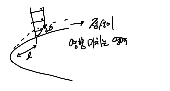
• A small area or region that viscosity dominates or influences
• BVP of thin boundary layer theory

Governing Equations

• Continuity eqn
• N.S with ${\partial p \over \partial y} = 0$

Boundary condition

• No-slip condition ($u=0, v=0$ on $y=0$)
• U, V potential flow velocity on far field $u=U, v=V$ on $y\to \infty$

Laminar vs Turbulant on Boundary layer

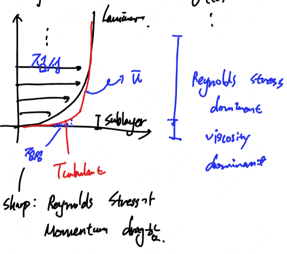
• A sharp sublayer exists on turbulant flow : Reynolds stress가 Momentum drag를 일으킴. → Viscosity가 dominant 한 영역을 줄여버림.
• Also, Turbulant boundary layer is Averaged line

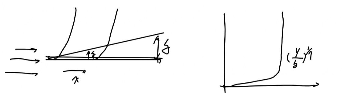
Dimensional analysis on Boundary Layer

• Define nondimensional variable

$x’ = x/l, y’= y/\delta, u’ = u/U, v’ = v/V$ : All nondimensional variables are order of one($\Theta(1)$)

Applying it to continuity eqn :

\[{u\partial u' \over l \partial x} + {v\partial v' \over \delta \partial y'} = 0\]

$\Theta({U\over l}) = \Theta({V\over \delta}) $ →$\Theta({\delta \over l}) = \Theta({V\over U}) $

Whch means..

IF $U»V$, $\delta « l$. makes thin boundary Layer

Definitions of Threee Boundary layer thicknesses

1. Boundary Layer thickness $\delta$ : $0.99u$에 도달하는 두께
2. Displacement thickness $\delta ^*$ :

\[\delta^* = \int_0^{\infty}(1-{u\over L})dy\]

• Displacement thickness 만큼
  1. Momentum thickness $\theta$ :

\[\theta = \int_0^\infty {u\over L} (1-{u\over L}) dy\]

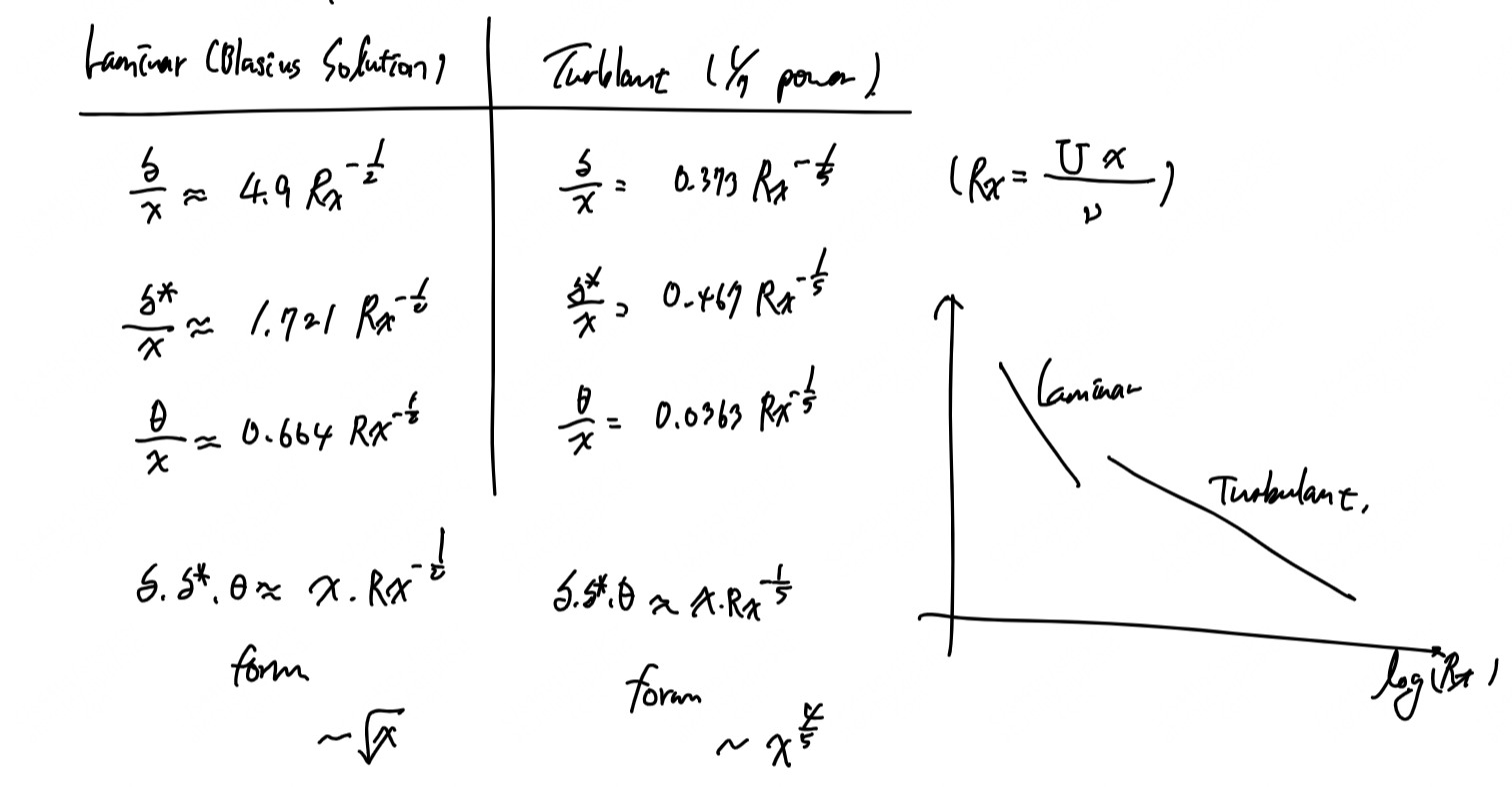
• Laminar condition, boundary layer thicknesses depends on 1/2 power of x
• In turbulant condition, thickness depends on 4/5 pwr of x

Skin friction coeff local

\[C_F = {\tau \over {1\over 2}\rho U^2}, C_{F,L} = 0.664Rx^{-0.5}, C_{F,T} = 0.0592Rx^{-0.5}\]

skin friction coefficient depends on length x, so

\[{1\over L} \int_0^L C_F dx = C_{F, Mean}\]

• Drag Force = Viscous drag + Residual drag
• Viscous drag = Friction drag on W.S. + form pressure drag

Viscous drag

\[C_D = {F_V\over {1\over 2}\rho A_{proj}U^2}\] \[\text{Viscous Drag} = {1\over 2} \rho C_D A_{proj} U\vert U\vert\]